MPI Deployment & Scalability
The Message Passing Interface deployed across the Pi 3 workers, used to demonstrate both Amdahl's Law (strong scaling) and Gustafson's Law (weak scaling) with two independent MPI example pairs: a compute-bound Monte Carlo π estimator and a communication-heavy matrix–vector multiplication.
What was asked
Deploy MPI on the cluster using Pi 3 nodes as workers and a Pi 4/5 as master. Demonstrate cluster scalability, analyze performance bottlenecks, and illustrate Amdahl's Law and Gustafson's Law using at least two MPI applications.
Theoretical background
Both laws describe the speedup S from running on p processes:
- p: number of processes.
- f: serial share of the work, the part that can't be split across processes.
- N: problem size (matrix rows, or samples for Monte Carlo). Fixed for Amdahl, grows with p for Gustafson.
Problem size is fixed. Adding processes gives less and less benefit, and speedup can
never go above 1/f, no matter how many processes you add.
Problem size grows with the number of processes, so each process always does the same amount of work. The serial part matters less as the problem grows, so speedup keeps rising.
What was built
MPI (Message Passing Interface, here OpenMPI) is a standardized protocol for
exchanging data across distributed-memory systems via explicit messages between
processes. OpenMPI and GCC were installed on the Pi 5 master and all 8 Pi 3 workers
(00_setup_all_nodes.sh). The four programs below are compiled with
mpicc. Step-by-step cluster setup:
MPI/task_3/task3_tutorial.md.
Four custom C programs across two example pairs, driven by a setup/run/analyse script pipeline and a hostfile giving each of the 8 Pi 3 workers exactly 4 slots (one per core):
montecarlo_amdahl.c/montecarlo_gustafson.c: Monte Carlo π estimation. Draws N random points(x, y)in the square from −1 to 1 on each side, and counts how many land inside the unit circle (wherex² + y² ≤ 1); that fraction times 4 estimates π. For the Amdahl run, N = 20,000,000 total points are split across processes, so more processes means fewer points each. For the Gustafson run, each process always draws the same 2,000,000 points, so more processes means a bigger total N. Embarrassingly parallel either way: each rank draws its own points locally, then sends just that one number (a singlelong, its local hit count) via oneMPI_Reducecall. However many points a rank drew, it always sends the same one number, so the message size stays O(1) regardless of N or p. Only the local compute work scales.amdahl_matrix.c/gustafson_matrix.c: matrix–vector multiplication. Multiplies an N×N matrix by a vector of the same length N.N = 1500and fixed for the Amdahl run.N = 150 → 4800and growing with p for the Gustafson run. The matrix rows are split across processes. Both compute and communication scale as O(N²), so this pair is the one deliberately used to expose the cluster's communication/memory-bandwidth limits.
Why p = 1, 2, 4, 8, 12, …, 32 and not 1, 2, 3, 4, …:
each Pi 3 gets exactly 4 slots, so p = 4, 8, 12, … each correspond to using
exactly 1, 2, 3, … complete physical nodes: every step adds one whole Pi 3, which makes it
possible to attribute changes in the data to node count rather than an uneven, partial split
of cores. p = 1 and p = 2 additionally test partial use of the
first node's 4 cores, deliberately making the within-node effect visible before the first
full node is reached.
Amdahl's Law: strong scaling
Full analysis: MPI/task_3/results/mpi_benchmark_report.md.
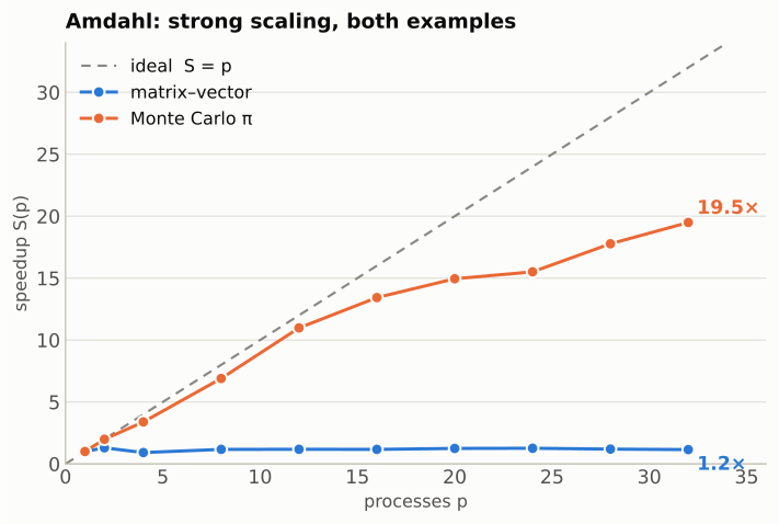
Monte Carlo π, fixed at 20,000,000 samples, is the clearer demonstration of the law itself. It still loads every worker's CPU with real computation, but its O(1) communication never stresses the network or memory bus, so the curve follows the textbook diminishing-returns shape closely.
| p | Wall time (s) | Measured speedup | Efficiency |
|---|---|---|---|
| 1 | 23.018 | 1.000 | 100.0% |
| 2 | 11.578 | 1.988 | 99.4% |
| 4 | 6.791 | 3.390 | 84.7% |
| 8 | 3.336 | 6.899 | 86.2% |
| 16 | 1.714 | 13.429 | 83.9% |
| 32 | 1.181 | 19.491 | 60.9% |
The matrix-vector control: a real hardware ceiling
The matrix-vector variant (fixed N = 1500, 200 iterations) hits a measured
ceiling far below linear: S(32) ≈ 1.15× at just 3.6% efficiency.
Adding processes buys almost nothing past the first few. Compute-only time barely improves
from p=1 to p=4 (0.01141 s → 0.01151 s per iteration, averaged over
200 iterations), even though all four processes share one physical Pi 3's 4 cores. Matrix–vector
multiplication is memory-bound: lots of RAM traffic per arithmetic op, little reuse. Our
reading is that all 4 cores are saturating the Pi 3's single shared memory bus. Memory-bus
utilisation itself wasn't instrumented, so this is our best explanation for the flat timing,
not a confirmed measurement of the bus. In fact the single biggest step in the whole speedup
series is a drop, from p=2 to p=4 (1.297× → 0.916×, below the
p=1 baseline), happening entirely within one Pi 3, which lines up with that same
bus-contention reading. Speedup then partially recovers at p=8 (0.916× → 1.171×)
once a second physical node joins, consistent with, but (measured only once) not proof of, a
switch from local memory copies to real Ethernet transfer for the scatter/gather.
Directly comparing the two: Monte Carlo π reaches 19.5× at p=32 vs. the matrix variant's 1.15× on identical hardware. That is strong evidence that the matrix bottleneck is algorithm-specific (driven by its O(N²) communication), not a hard ceiling of the cluster itself.
Gustafson's Law: weak scaling
Problem size grows with process count instead of staying fixed, so each process keeps a constant amount of work.
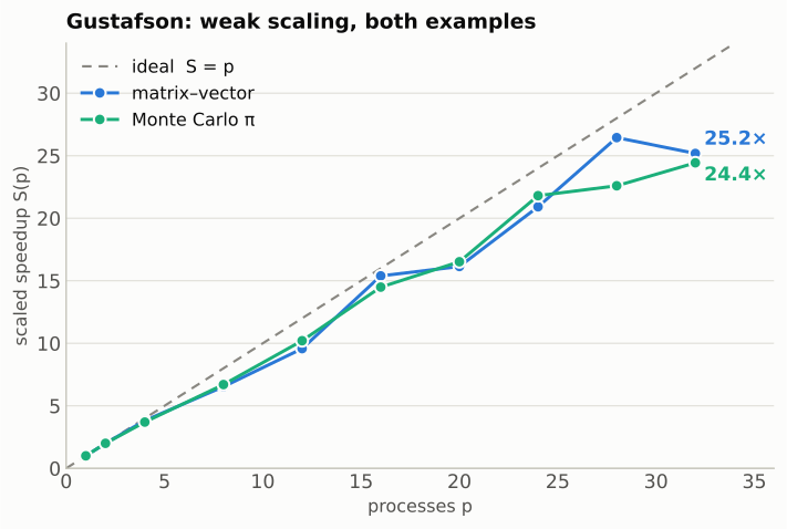
Both examples land in a similar range here, despite Monte Carlo's O(1) payload vs. the
matrix variant's O(N) result-vector gather, which on its own would suggest Monte Carlo
should be clearly lower. f_serial in both is measured directly per run (not
fitted), so the closeness is real. Our reading is that in both cases it's dominated by
MPI_Barrier/MPI_Reduce-style synchronisation latency (rank 0
waiting for the slowest of the heterogeneous Pi3 nodes) rather than by payload size. We did
not capture per-rank timing to confirm this directly. Efficiency at p=32 is
76.4% (Monte Carlo) vs. 78.7% (matrix), a further sign both are limited by something other
than data volume.
Why N = 1500, not larger (matrix-vector)
Compute and communication both scale as O(N²) for matrix–vector multiplication, so
the ratio between them doesn't fundamentally improve with larger N. It only
makes every run take longer. A test at N = 5000 (30 iterations) confirmed this
empirically: it performed worse than the N = 1500 result, because 30
iterations weren't enough to amortise the ~11× larger one-time transfer cost (18 MB → 200 MB)
at that size. This is one confirmation test, not a sweep across many N values, so it
supports rather than fully proves the general O(N²) argument above.
Conclusion
Both laws were demonstrated with real measured data across two independent example pairs: Monte Carlo π shows the textbook Amdahl/Gustafson curve shape on hardware that isn't the bottleneck, while matrix-vector multiplication exposes a real, measured hardware ceiling (S(32) ≈ 1.15×, 3.6% efficiency) that Monte Carlo confirms is algorithm-specific rather than a cluster-wide limit. Where a claim goes beyond what's directly measured (e.g. attributing a pattern to the shared memory bus or to synchronisation latency), it's flagged as interpretation above, since no per-rank timing or hardware bus/network counters were captured.