Task 4

Scaling Laws — Non-MPI Demonstration

PovRay/ ("pi-scaling-lab")

A from-scratch POV-Ray rendering harness that demonstrates Amdahl's and Gustafson's Laws without MPI.

What was asked

Demonstrate Amdahl's Law and Gustafson's Law using a non-MPI tool such as Task Distributor.

Theoretical background

Both laws describe the speedup S on N nodes for a workload whose P is the parallel fraction — the share of the work that can actually be split.

Amdahl S(N) = 1 (1 − P) + P/N ceiling: 1 / (1 − P)

The problem size is fixed, so adding nodes gives diminishing returns and speedup can never exceed 1/(1−P) no matter how many nodes you add.

Gustafson S(N) = (1 − P) + P · N no ceiling: grows with N

If the problem grows with the node count, the serial part becomes an ever smaller share of the total work, so speedup keeps rising with N and parallelisation stays worthwhile.

In this project, Amdahl is shown by rendering a fixed image on N = 1…8 nodes at three image sizes, and Gustafson by growing the image with N so that every node always renders the same number of rows.

What was built

One harness, src/povbench.py — pure Python standard library on the worker nodes, no MPI and no external dependencies. It splits a POV-Ray render by image rows across nodes to measure strong scaling (Amdahl) and weak scaling (Gustafson), with per-phase timing so the sequential fraction is measured, not just curve-fitted.

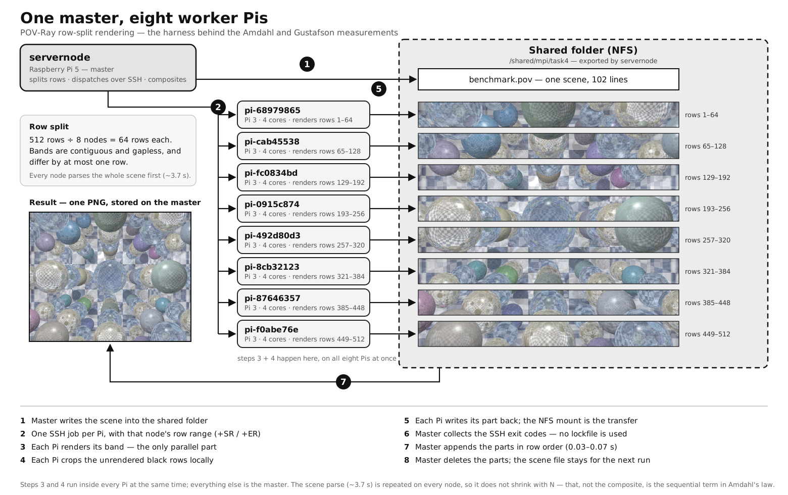
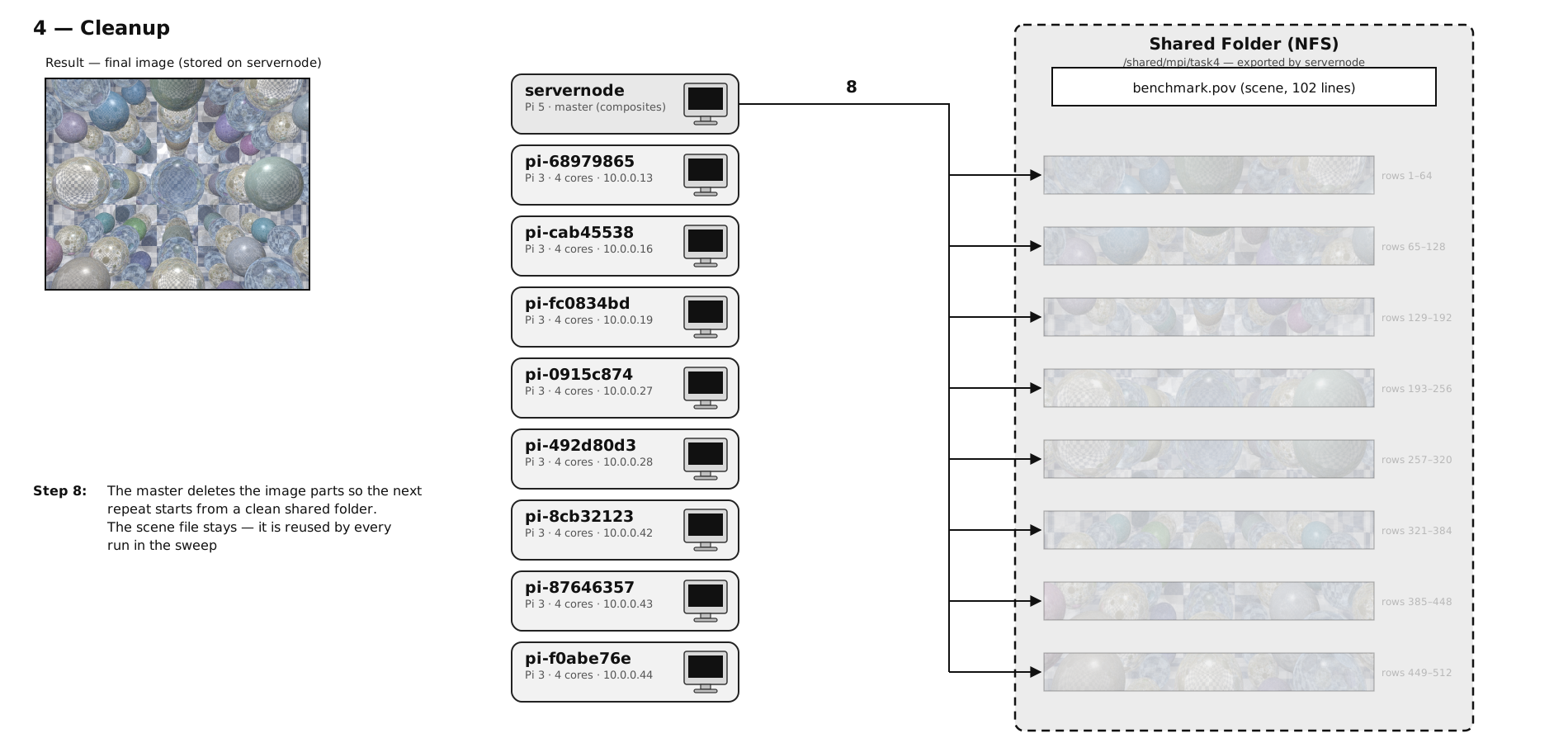
One master and eight worker Pis render a single POV-Ray scene by splitting it into horizontal bands of rows. The scene file is written once into the shared NFS folder; each node renders only its own band.

Poster overview: one master and eight worker Pis, each rendering a 64-row band of the same POV-Ray scene from a shared NFS folder — **Poster overview.** Row-split rendering across the cluster — the harness behind the Amdahl and Gustafson measurements. Click the figure to open it full size.

How a run executes

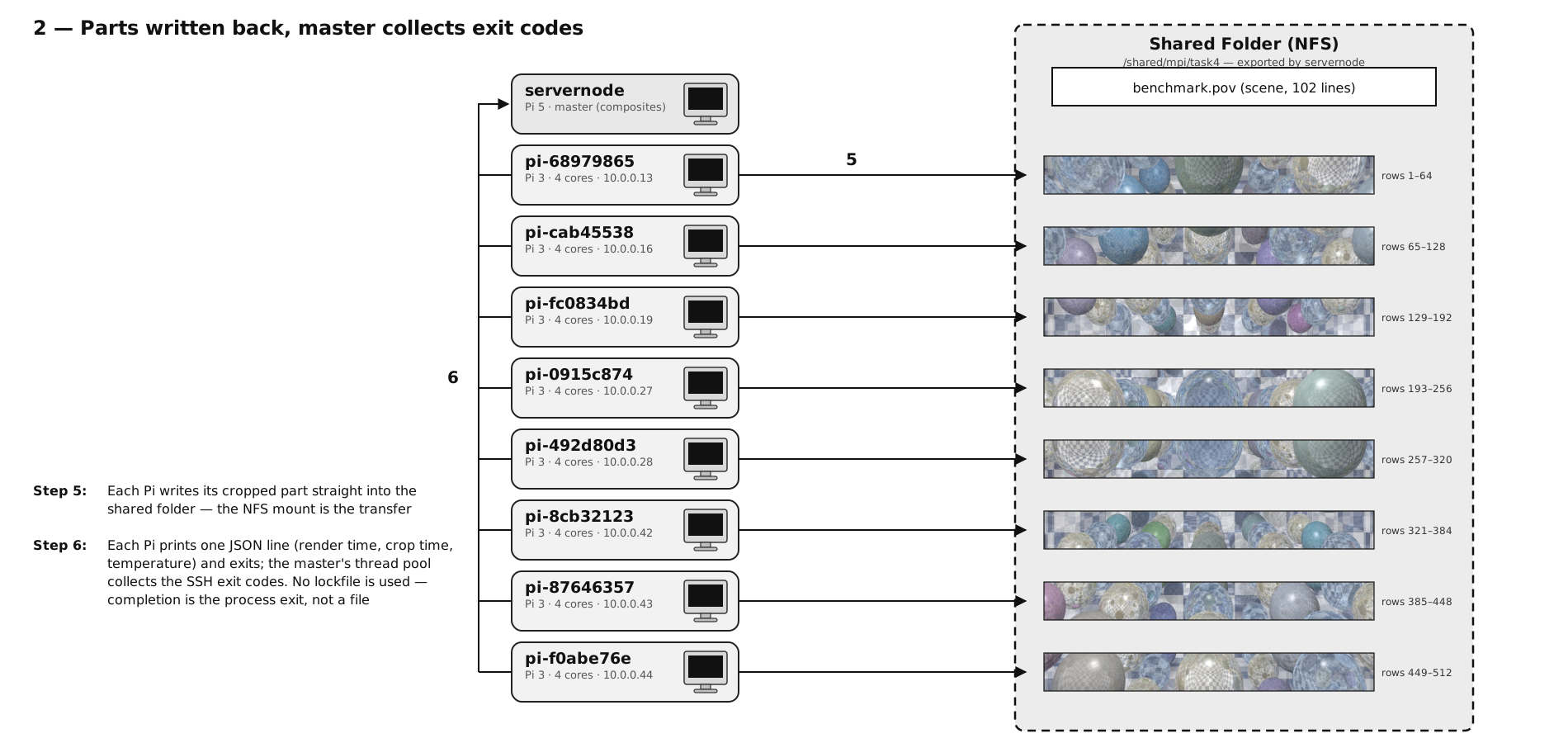
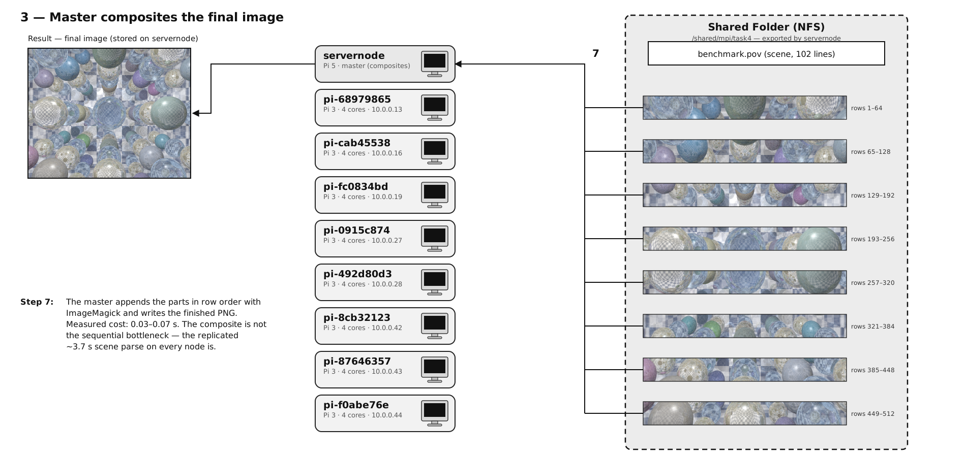
Eight steps, grouped into four phases. Each phase is timed separately, which is what makes the sequential fraction a measured quantity rather than a fitted one.

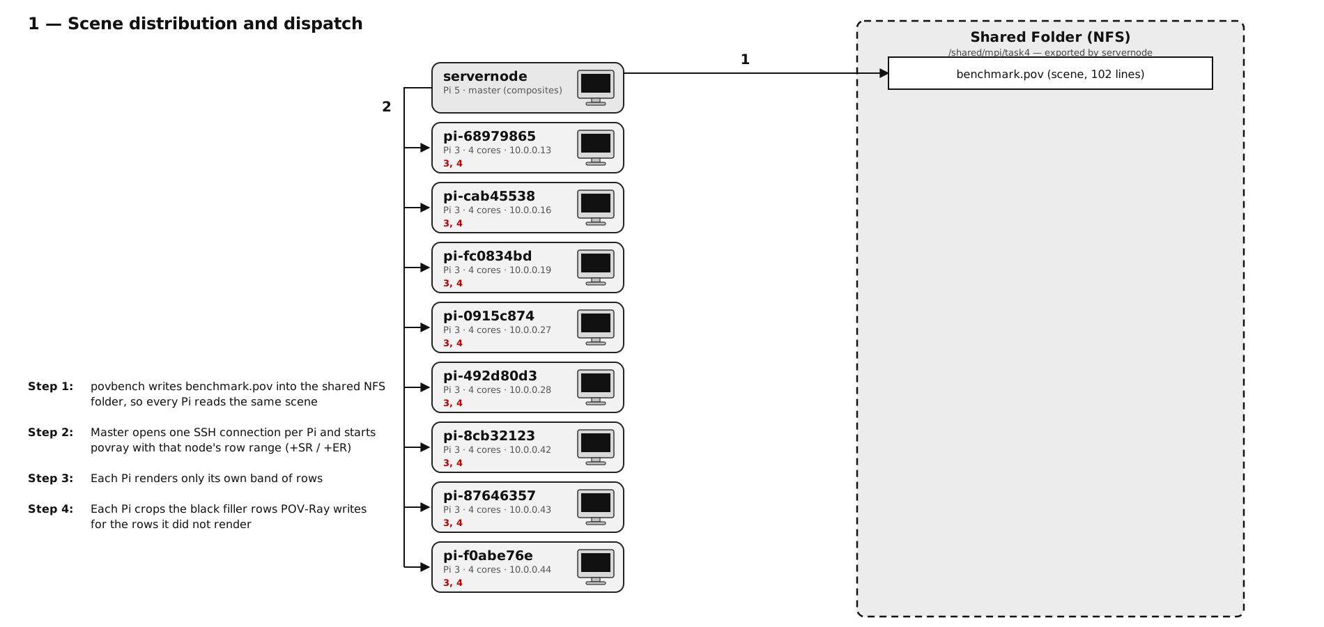
Workflow phase 1: the master writes the scene to NFS, opens one SSH connection per Pi with a row range, and each Pi renders and crops its own band — **1 — Scene distribution and dispatch.** `povbench` writes `benchmark.pov` into the shared NFS folder so every Pi reads the same scene; the master opens one SSH connection per Pi and starts `povray` with that node's row range (`+SR`/`+ER`); each Pi renders its band and crops the black filler rows POV-Ray writes. Steps 1–4. Click to open full size.

Workflow phase 2: each Pi writes its cropped part into the shared folder and prints a JSON timing line; the master collects SSH exit codes — **2 — Parts written back, exit codes collected.** Each Pi writes its cropped part straight into the shared folder — the NFS mount is the transfer — then prints one JSON line (render time, crop time, temperature) and exits. No lockfile: completion is the process exit, not a file. Steps 5–6. Click to open full size.

Workflow phase 3: the master appends the parts in row order with ImageMagick and writes the finished PNG — **3 — Master composites the final image.** The parts are appended in row order with ImageMagick. Measured cost: 0.03–0.07 s — so the composite is *not* the sequential bottleneck. The replicated ~3.7 s scene parse on every node is. Step 7. Click to open full size.

Workflow phase 4: the master deletes the image parts, leaving the scene file in the shared folder for the next repeat — **4 — Cleanup.** The master deletes the image parts so the next repeat starts from a clean shared folder. The scene file stays — every run in the sweep reuses it. Step 8. Click to open full size.

Finding The phase timings put the composite at well under a tenth of a second, while every node pays the same ~3.7 s scene parse before it renders a single row. The (1−P) term is therefore dominated by replicated setup, not by the master’s serial join — which is exactly the kind of disagreement between fitted and measured P that a single wall-clock number would have hidden.

Why not just wrap Task-Distributor

Task-Distributor's master script does dispatch, wait, and composite in one block, producing a single wall-clock number per run — leaving you to fit P after the fact to make the curve look right. This harness reimplements the same row-splitting approach (Rooney's method: POV-Ray +SR/+ER, crop black filler rows on the worker, -append on the master) but wraps a timer around each phase. The composite step on the master is the (1−P) term in Amdahl's Law — measuring it directly means the fitted P can be checked against a measured one. When they disagree, that disagreement is itself a finding.

Measurement protocol

Every run in the sweep was taken under these rules; each one exists because of a specific failure mode encountered on this cluster:

≥30 s cooldown between runs — so a heat-soaked cluster does not carry throttling from one run into the next.
≥3 repetitions per configuration, reported as the median — a mean would let a single throttled run invent a bend in the curve.
Run order randomised within each image size — sweeping N=1→8 in sequence would make thermal drift correlate with node count and mimic parallelisation overhead.
performance governor pinned on the workers — the default ondemand governor adds variance to every timing.
Temperature and throttle state logged per run, classified as clean / sticky / active — only active capping invalidates a run, sticky flags latch until reboot.
NFS cache warmed before timing — a cold worker's first band reads POV-Ray's .inc files over NFS and is a one-off 3.82 s against 2.3 s.

Results

Amdahl — the ceiling moves with the problem size

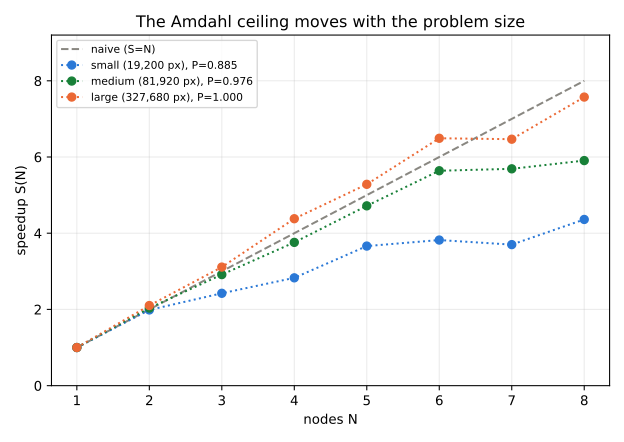
Speedup against node count for three image sizes; the small image flattens early while the large one tracks the ideal line — **Strong scaling at three image sizes**, N = 1…8, median of 3 runs. Fitted parallel fraction P in the legend. Click the figure to open it full size.

Size	Pixels	T(1)	T(8)	Speedup	Fitted P	Ceiling
small	19,200	51.39 s	11.78 s	4.36×	0.885	8.7×
medium	81,920	170.35 s	28.84 s	5.91×	0.976	41.1×
large	327,680	592.33 s	78.21 s	7.57×	1.000	off-scale

Gustafson — the line rises, and the rise is accounted for

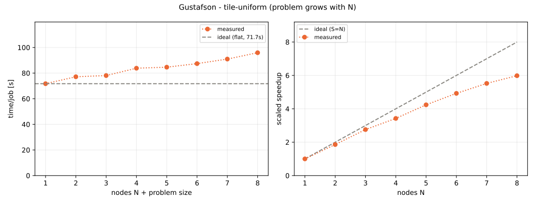
Weak scaling: time per job rises gently from 71.7 s to 95.9 s as nodes and problem size grow together, and scaled speedup reaches 5.98 against an ideal of 8 — **Weak scaling** (`scene --weak`, 1024 × 2048 rows per node, N = 1…8, median of 3). Scaled speedup 5.98× at N=8, fitted P = 0.759, R² = 0.988. Click the figure to open it full size.

Time per job rises 33.7 % (71.73 s → 95.91 s) instead of staying flat, and both mechanisms were measured rather than inferred: +14.59 s of load imbalance from node heterogeneity, and +9.56 s of composite growth on the master, whose output image grows with N. Together they explain 24.15 s of the 24.18 s deviation. The first attempt at this measurement was invalid; see why the first weak-scaling scene was wrong.

Problems encountered

Thermal throttling on the master. The Pi 5 ran continuously at 89–90 °C and 1.0 GHz against a 2.4 GHz maximum, which inflated the measured serial term.
Thermal throttling on the workers. Sustained renders pushed the Pi 3 workers to ~78 °C and into the soft temperature limit.
The first Gustafson run was invalid. Growing the strong-scaling scene taller made the added rows far cheaper than the central ones, so the work per node was not constant — fixed with an orthographic weak-scaling scene.

Side-by-side comparison: the broken scene shows band render times from 1.10 s to 5.75 s across eight Pis (4.76x spread), the fixed weak-scaling scene shows 0.13-0.15 s across all eight (1.06-1.11x spread) — **Why the first weak-scaling scene was wrong.** One frame split into the eight bands the eight Pis render at N=8; bar length is that band's render time. Left: the strong-scaling scene grown taller — **4.76× spread**. 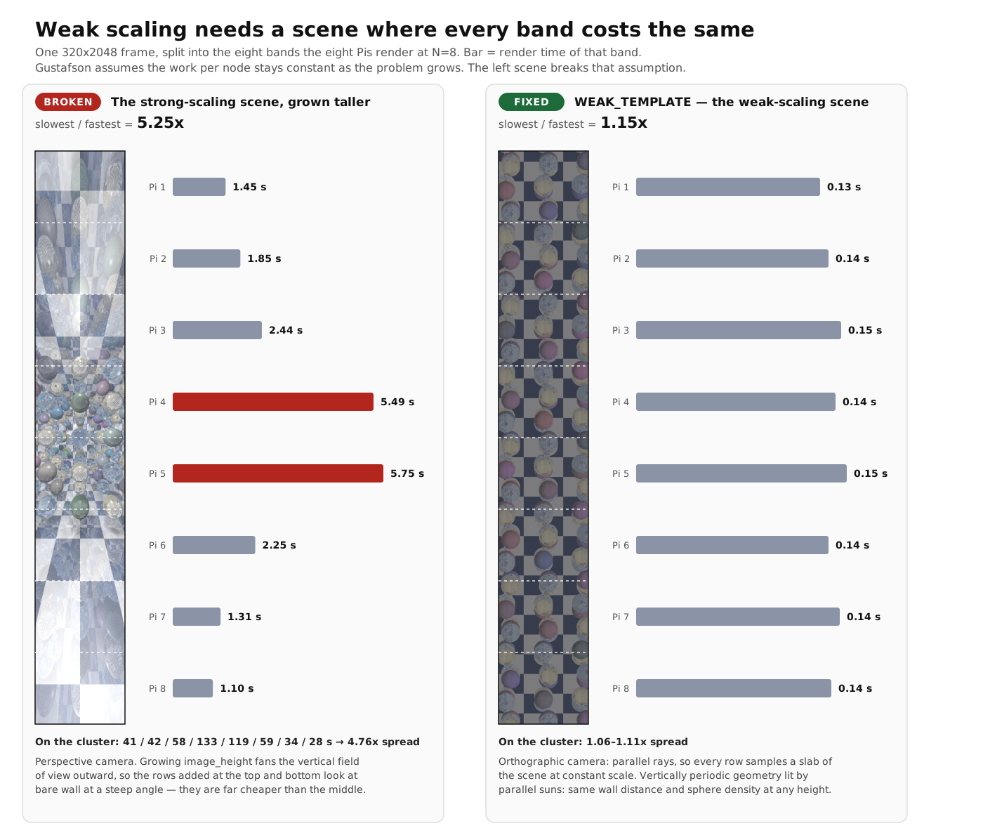Right: the `--weak` scene — **1.06–1.11×**. Click the figure to open it full size.

Reproducing it

The harness runs on the Pi 5 master (10.0.0.1) — the only machine with a foot in both the tailnet and the isolated 10.0.0.0/24 worker network. Workflow: author locally, rsync to the Pi 5, run there, pull results back — there is no git on the Pis, so the repository is the record of what ran.

Target	What it does
`make preflight`	checks clock skew, identity, thermal state, CPU governor, shared folder
`make install`	deploys the worker helper; verifies tools, installs nothing extra
`make scene`	builds the closed-room benchmark scene
`make plan` / `make run`	writes the run manifest and prints a time estimate, then executes (~3h; safe to Ctrl-C)
`make status` / `make resume`	check progress, continue later — even days later
`make analyze`	fits `P`, builds speedup tables, exports CSV + plots
`make selftest` / `make simulate`	offline correctness test, and a fast-forwarded virtual cluster for testing orchestration logic

Conclusion

Both laws were demonstrated without MPI, on a row-split POV-Ray render across eight Pi 3 workers. Amdahl was measured at three image sizes: the fitted parallel fraction rises with the problem size, moving the ceiling from 8.7× to 41.1× — the limit is a property of the workload, not of the cluster. Gustafson was measured with a vertically uniform scene so that every node does identical work, and the 33.7 % rise in time per job was decomposed into load imbalance and composite growth to within 0.03 s.

The per-phase timing is what made that possible. Because dispatch, render, transfer and composite were each timed separately, the sequential fraction could be compared against the fitted one instead of being inferred from it — which is how the replicated ~3.7 s scene parse, rather than the master’s composite step, was identified as the real limit on strong scaling.